Acid Precipitation and Remediation of Acid Lakes

Introduction

Acid precipitation has been a serious environmental problem in many areas of the world for the last few decades. Acid precipitation results from the combustion of fossil fuels which produce oxides of sulfur and nitrogen that react in the earth’s atmosphere to form sulfuric and nitric acid. One of the most significant impacts of acid rain is the acidification of lakes and streams. In some watersheds the soil doesn’t provide ample acid neutralizing capacity to mitigate the effect of incident acid precipitation. These susceptible regions are usually high elevation lakes with small watersheds and shallow non-calcareous soils. The underlying bedrock of acid-sensitive lakes tends to be granite or quartz. These minerals are slow to weather and therefore have little capacity to neutralize acids. The relatively short contact time between the acid precipitation and the watershed soil system exacerbates the problem. Lakes most susceptible to acidification: 1) are located downwind, sometimes hundreds of miles downwind, from major pollution sources–electricity generation, metal refining operations, heavy industry, large population centers, etc.; 2) are surrounded by hard, insoluble bedrock with thin, sandy, infertile soil; 3) have a high runoff to infiltration ratio; 4) have a low watershed to lake surface area. Isopleths of precipitation pH are depicted in Fig. 4.

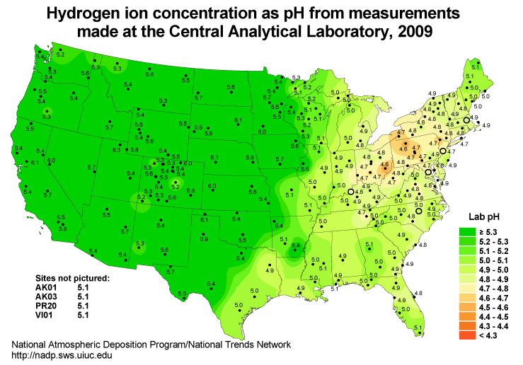
Fig. 4 The pH of precipitation in 2009.

In acid-sensitive lakes the major parameter of concern is pH (\(pH = -log{\{H^+\}}\), where \(\{H^+\}\) is the hydrogen ion activity, and activity is approximately equal to concentration in moles/L). In a healthy lake, ecosystem pH should be in the range of 6.5 to 8.5. In most natural freshwater systems, the dominant pH buffering (controlling) system is the carbonate system. The carbonate buffering system is composed of four components: dissolved carbon dioxide (\({CO}_{{2\; aq}}\)), carbonic acid (\({H}_{{2}} {CO}_{{3}}\)), bicarbonate (\({HCO}_{{3}}^{{-}}\)), and carbonate (\({CO}_{{3}}^{{-2}}\)). Carbonic acid exists only at very low levels in aqueous systems and for purposes of acid neutralization is indistinguishable from dissolved carbon dioxide. Thus to simplify things we define

(4)\[ \left[{H}_{{2}} {CO}_{{3}}^{{*}} \right]=\left[{CO}_{{2\; aq}} \right]+\left[{H}_{{2}} {CO}_{{3}} \right]\]

The \(\left[{CO}_{{2\; aq}} \right] \mathrm{>} \mathrm{>} \left[{H}_{{2}} {CO}_{{3}} \right]\) and thus \(\left[{H}_{{2}} {CO}_{{3}}^{{*}} \right]\cong \left[{CO}_{{2\; aq}} \right]\) (all terms enclosed in [] are in units of moles/L).

The sum of the molar concentrations of all the components of the carbonate system is designated as \(C_T\) as shown in the equation below.

(5)\[C_T = \left[H_2{CO}_3^* \right] + \left[{HCO}_3^- \right]+\left[{CO}_3^{-2} \right]\]

The carbonate system can be considered to be a “volatile” system or a “non-volatile” system depending on whether or not aqueous carbon dioxide is allowed to exchange and equilibrate with atmospheric carbon dioxide. Mixing conditions and hydraulic residence time determine whether an aquatic system is volatile or non-volatile relative to atmospheric carbon dioxide equilibrium. First, consider the relationship that are valid regardless of the rate of exchange with the atmosphere.

Carbonate System

For a fixed \(C_T\), the molar concentration of each species of the carbonate system is determined by pH. Equations (6)-(11) show these functional relationships.

(6)\[ \left[H_2 {CO}_3^* \right] = \frac{C_T}{1+\frac{K_1}{[H^+]} +\frac{K_1 K_2}{[H^+]^2} } = \alpha_0 C_T\]

where

(7)\[ \alpha_0 =\frac{1}{1+\frac{K_1 }{[H^+]} +\frac{K_1 K_2}{[H^+]^2} }\]

(8)\[ \left[{HCO}_3^- \right]=\frac{C_T}{\frac{[H^+ ]}{K_1 } +1+ \frac{K_2}{[H^+]}} =\alpha_1 C_T\]

where

(9)\[ \alpha_1 = \frac{1}{\frac{[H^+]}{K_1} + 1 + \frac{K_2}{[H^+]}}\]

(10)\[ \left[{CO}_3^{-2} \right] = \frac{C_T}{\frac{[H^+]^2}{K_1 K_2} +\frac{[H^+]}{K_2} +1 } =\alpha_2 C_T\]

where

(11)\[ \alpha_2 = \frac{1}{\frac{[H^+]^2 }{K_1 K_2} +\frac{[H^+]}{K_2} + 1}\]

\(K_1\) and \(K_2\) are the first and second dissociation constants for carbonic acid and \(\alpha_0\), \(\alpha_1\), and \(\alpha_2\) are the fraction of \(C_T\) in the form \(H_2CO_3^\star\), \(HCO_3^-\), and \(CO_3^{-2}\) respectively. Because \(K_1\) and \(K_2\) are constants (\(K_1 = 10^{-6.3}\) and \(K_2 = 10^{-10.3}\)), \(\alpha_0\), \(\alpha_1\), and \(\alpha_2\) are only functions of pH.

A measure of the susceptibility of lakes to acidification is the acid neutralizing capacity (ANC) of the lake water. In the case of the carbonate system, the ANC is exhausted when enough acid has been added to convert the carbonate species \({HCO}_{{3}}^{{-}}\) and \({CO}_{{3}}^{{-2}}\) to \({H}_{{2}} {CO}_{{3}}^\star\). A formal definition of total acid neutralizing capacity is given by equation (12)

(12)\[ {ANC\; }={\; }\left[{HCO}_{{3}}^{{-}} \right]+{\; 2}\left[{CO}_{{3}}^{{-2}} \right]+\left[{OH}^{{-}} \right]{\; -}\left[{H}^{+} \right]\]

ANC has units of equivalents per liter. The hydroxide ion concentration can be obtained from the hydrogen ion concentration and the dissociation constant for water, \(K_w\).

(13)\[ \left[{OH}^{{-}} \right] = \frac{K_w}{\left[H^+\right]}\]

Substituting equations (8), (10), and (13) into equation (12), we obtain

(14)\[ ANC=C_T \left(\alpha_1 +2\alpha_2 \right)+\frac{K_w}{\left[H^+ \right]} - \left[H^+ \right]\]

For the carbonate system, ANC is usually referred to as alkalinity. Alkalinity can be expressed as equivalents/L or as mg/L (ppm) of \(CaCO_3\). 50,000 mg/L \(CaCO_3\) = 1 equivalent/L.

Volatile Carbonate Systems

Now consider the case where aqueous \({CO}_{2\; aq}\) is volatile and in equilibrium with atmospheric carbon dioxide. Henry’s Law can be used to describe the equilibrium relationship between atmospheric and dissolved carbon dioxide.

(15)\[\left[{CO}_{{2\; aq}} \right]={\; P}_{{CO}_{{2}} {\; }} {K}_{{H}}\]

where \(K_H\) is Henry’s constant for \(CO_2\) in moles/L-atm and \(P_{CO_2}\) is partial pressure of \(CO_2\) in the atmosphere \(K_H = 10^{-1.5}\) and \(P_{CO_2} = 10^{-3.5}\)). Because \(\left[{CO}_{{2\; aq}} \right]\) is approximately equal to \(\left[H_2CO_3^{\star} \right]\) and from equations (4) and (6)

(16)\[P_{CO_2} K_H =\alpha_0 C_T\]

(17)\[ C_T = \frac{P_{CO_2} K_H}{\alpha_0}\]

Equation (17) gives the equilibrium concentration of carbonate species as a function of pH and the partial pressure of carbon dioxide.

The acid neutralizing capacity expression for a volatile system can be obtained by combining equations (17) and (14).

(18)\[ ANC=\frac{P_{CO_2} K_H }{\alpha_0 } (\alpha_1 +2\alpha_2 ) + \frac{K_w }{\left[H^+ \right]} - \left[H^+ \right]\]

In both non-volatile and volatile systems, equilibrium pH is controlled by system ANC. Addition or depletion of any ANC component in equation (14) or (18) will result in a pH change. Natural bodies of water are most likely to approach equilibrium with the atmosphere (volatile system) if the hydraulic residence time is long and the body of water is shallow.

Lake ANC is a direct reflection of the mineral composition of the watershed. Lake watersheds with hard, insoluble minerals yield lakes with low ANC. Typically watersheds with soluble, calcareous minerals yield lakes with high ANC. ANC of freshwater lakes is generally composed of bicarbonate, carbonate, and sometimes organic matter (\({A}_{{org}}^{{-}}\)). Organic matter derives from decaying plant matter in the watershed. When organic matter is significant, the ANC becomes (from equations (14) and (18)):

(19)\[ ANC=C_{T} (\alpha _{1} +2\alpha _{2} )+{\; }\frac{K_{w} }{\left[{H}^{+} \right]} \; -\left[{H}^{+} \right]+\left[{A}_{{org}}^{{-}} \right]\]

(20)\[ ANC=\frac{P_{CO_{2} } K_{H} }{a_{0} } (\alpha _{1} +2\alpha _{2} )+\frac{K_{w} }{\left[{H}^{+} \right]} \; -\left[{H}^{+} \right]+\left[{A}_{{org}}^{{-}} \right]\]

where equation (19) is for a non-volatile system and equation (20) is for a volatile system.

During chemical neutralization of acid, the components of ANC associate with added acid to form protonated molecules. For example:

(21)\[\left[{H}^{+} \right]{\; }+{\; }\left[{HCO}_{{3}}^{{-}} \right]{\; }\to \; \left[{H}_{{2}} {CO}_{{3}}^{{\star}} \right]\]

or

(22)\[\left[{H}^{+} \right]{\; }+{\; }\left[{A}_{{org}}^{{-}} \right]{\; }\to \; \left[{HA}_{{org}} \right]\]

In essence, the ANC of a system is a result of the reaction of acid inputs to form associated acids from basic anions that were dissolved in the lake water. The ANC (equation (12)) is consumed as the basic anions are converted to associated acids. This conversion is near completion at low pH (approximately pH 4.5 for the bicarbonate and carbonate components of ANC). Neutralizing capacity to another (probably higher) pH may be more useful for natural aquatic systems. Determination of ANC to a particular pH is fundamentally easy — simply add and measure the amount of acid required to lower the sample pH from its initial value to the pH of interest. Techniques to measure ANC are described under the procedures section of this lab.

Neutralization of acid precipitation can occur in the watershed or directly in the lake. How much neutralization occurs in the watershed versus the lake is a function of the watershed to lake surface area. Generally, watershed neutralization is dominant. Engineered remediation of acid lakes has been accomplished by adding bases such as limestone, lime, or sodium bicarbonate to the watershed or directly to the lakes.

Reactor Theory Applied to Acid Lake Remediation

In this experiment sodium bicarbonate will be added to a lake to mitigate the deleterious effect of acid rain. Usually sodium bicarbonate is added in batch doses (as opposed to metering in). The quantity of sodium bicarbonate added depends on how long a treatment is desired, the acceptable pH range and the quantity and pH of the incident rainfall. For purposes of this experiment, a 15-minute design period will be used. That is, we would like to add enough sodium bicarbonate to keep the lake at or above its original pH and alkalinity for a period of 15 minutes (i.e., for one hydraulic residence time).

By dealing with ANC instead of pH as a design parameter, we avoid the issue of whether the system is at equilibrium with atmospheric carbon dioxide. Keep in mind that eventually the lake will come to equilibrium with the atmosphere. In practice, neutralizing agent dosages may have to be adjusted to take into account non-equilibrium conditions.

We must add enough sodium bicarbonate to equal the negative ANC from the acid precipitation input plus the amount of ANC lost by outflow from the lake during the 15-minute design period. Initially (following the dosing of sodium bicarbonate) the pH and ANC will rise, but over the course of 15 minutes, both parameters will drop. Calculation of required sodium bicarbonate dosage requires performing a mass balance on ANC around the lake. This mass balance will assume a completely mixed lake and conservation of ANC. Chemical equilibrium can also be assumed so that the sodium bicarbonate is assumed to react immediately with the incoming acid precipitation. Mass balance on the reactor yields:

(23)\[Q\left(ANC_{in} - ANC_{out} \right) \rlap{-} V \frac{d(ANC)}{dt}\]

where:

\(ANC_{out}\) = ANC in lake outflow at any time t (for a completely mixed lake the effluent ANC is the same as the ANC in the lake)

\(ANC_{in}\) = ANC of acid rain input

\(\rlap{-} V\) = volume of reactor

\(Q\) = acid rain input flow rate.

If the initial ANC in the lake is designated as ANC0, then the solution to the mass balance differential equation is:

(24)\[ANC_{out} \; =\; ANC_{in} \; \cdot \; \left(1\; -\; {\mathop{e}\nolimits^{-t/\theta \; \; }} \right)+\; ANC_{0} \; \cdot \; {\mathop{e}\nolimits^{-t/\theta \; }}\]

where:

\(\theta = \rlap{-} V/Q\)

We want to find ANC0 such that ANCout = 50 \(\mu eq/L\) when t is equal to \(\theta\). Solving for \(ANC_{0}\) we get:

(25)\[ {ANC}_{{0}} {\; }=\left[{ANC}_{out} - ANC_{in} \cdot \left(1 - {\mathop{e}\nolimits^{-t/\theta}} \right)\right]{\mathop{e}\nolimits^{t/\theta}}\]

The ANC of the acid rain (\(ANC_{in}\)) can be estimated from its pH. Below pH 6.3 most of the carbonates will be in the form \(H_2CO_3^{\star}\) and thus for pH below about 4.3 equation (12) simplifies to

(26)\[{ANC}\cong -\left[{H}^{+} \right]\]

An influent pH of 3.0 implies the \(ANC_{in} = -\left[H^+ \right] = -0.001 eq/L\)

Substituting into equation (25):

(27)\[{ANC}_{{0}} {\; }=\left[{0.000050}+{0.001\; }\cdot \left(1\; -\; {\mathop{e}\nolimits^{-1}} \right)\right]{\mathop{e}\nolimits^{1}} = 1.854 meq/L\]

The quantity of sodium bicarbonate required can be calculated from:

(28)\[[NaHCO_3]_0 =ANC_0\]

where \([NaHCO_3]_0\) = moles of sodium bicarbonate required per liter of lake water

(29)\[\frac{{1.854\; mmole\; NaHCO}_3 }{liter} {\times }\frac{{84\; mg\; NaHCO}_3 }{{mmole\; NaHCO}_3 } {\times \; 4\; Liters\; =\; 623\; mg\; NaHCO}_3\]

Experimental Objectives

Remediation of acid lakes involves addition of ANC so that the pH is raised to an acceptable level and maintained at or above this level for some design period. In this experiment sodium bicarbonate (\(NaHCO_3\)) will be used as the ANC supplement. Since ANC addition usually occurs as a batch addition, the design pH is initially exceeded. ANC dosage is selected so that at the end of the design period pH is at the acceptable level. Care must be taken to avoid excessive initial pH — high pH can be as deleterious as low pH.

The most common remediation procedure is to apply the neutralizing agent directly to the lake surface, instead of on the watershed. We will follow that practice in this lab experiment. Sodium bicarbonate will be added directly to the surface of the lake that has an initial ANC of \(0 \mu eq/L\) and is receiving acid rain with a pH of 3. After the sodium bicarbonate is applied, the lake pH and ANC will be monitored for over two approximately 20 minute periods.

Experimental Apparatus

The experimental apparatus consists of an acid rain storage reservoir, peristaltic pump, and lake (Fig. 5). The pH of the lake will be monitored using a pH probe connected to a signal-conditioning box that is connected to ProCoDA.

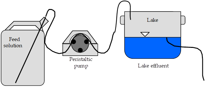
Fig. 5 Schematic drawing of the experimental setup.

procedures

The following directions are written for the use of ProCoDA II hardware and software for pH data collection and manual control of the peristaltic pump. It would also be possible to automate the experiment and control the pump using the ProCoDA II hardware and software.

We will use a pH probe to measure pH in this experiment. Each bench has one pH probe. Plug the pH probe into the blue signal-conditioning box (it takes a push and a twist). Connect the blue signal conditioning box to one of the sensor ports on your ProCoDA box.

Noisy pH measurements are a serious problem due to the static electricity generated by the peristaltic pump as it rotates and compresses the pump tubing. This can be solved by grounding the acidic solution as it is being pumped into the lake.

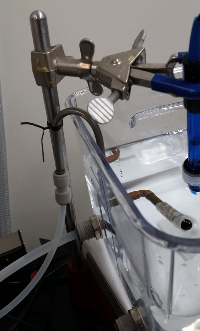
Fig. 6 Photo of the experimental setup showing how the incoming flow of acid is grounded to the metal rod that is connected to the stir plate that is electrically grounded. This prevents pH fluctuations caused by static electricity generated by the peristaltic pump.

It is important that the electrical connection be solid all the way from the inverted U tube to the ground wire that is connected to the building electrical system. If the pH probe is noisy it may be necessary to tighten one or more of the connections in that path.

1. Setup and calibrate the pH probe
2. Save the Calibration you have just created as a backup. You can do this by clicking on the button on the main menu.
3. Verify that the experimental setup is plumbed so that the acid rain is pumped directly into the lake. The lake outflow should discharge into the small drain on the side of your work bench.
4. Organize the bench setup so that the metal tube discharging the acid rain into the lake is solidly touching the metal stand that is connected to the stirrer. This will ground the solution that is in the lake and reduce voltage fluctuations that are easily measured by the pH probe.
5. Check all of the push to connect fittings. To obtain a water tight connection it is necessary to twist and push so that the o’ring slides over the outside of the tube to create a seal. You can test run your system with just reverse osmosis water to check for leaks.
6. Preset pump to give desired flow rate of 267 mL/min (4 L/15 minutes) based on the size of pump tubing selected. Do not turn the pump on yet! For each tubing size, different pump speeds will correspond to different flow rates being output by the pump. The peristaltic tubing sizes are rather arbitrary and are labeled by numbers: 13, 14, 16, 17, and 18 in increasing order of size. If you have #18 tubing, you will want an RPM setting of (267 mL/min) / (3.8 mL/rev) = 70.3 RPM (see Table 11).
7. Fill lake with reverse osmosis water and verify that the outflow is set so the lake volume is approximately 4 L. Place the lake on top of a magnetic stirrer and add a stir bar.
8. Set stirrer speed to 8.
9. Add 1 mL of bromocresol green indicator solution to the lake.
10. Weigh out 623 mg (not grams!) \(NaHCO_3\).
11. Add \(NaHCO_3\) to the lake.
12. After the lake is well stirred take a 100 mL sample from the lake in the plastic sample bottle on your bench (this does not have to be exactly 100 mL; you just need enough for a pH reading). Don’t forget to label the sample bottle (include the time of the sample ex. Minute 0).
13. Clip the pH probe to the side of your lake in a more quiescent zone, away from the influent and effluent. You can do this with a clamp or you can simply tape the pH probe cable to the side of your lake.
14. We will continuously measure the pH of the effluent and log the data into a tab delimited file. Set the data interval to 1 second. Begin logging data to file by clicking on the button. Create a new file in S:\Courses\4530\Group #\Lab 2 – Acid Rain.
15. Prepare to write a comment in the file to mark the time when the pump starts by clicking on the button. Type in a comment and then wait (the comment will not show up on the data sheet until you click enter).
16. At time equal zero (t=0) start the peristaltic pump and click on the enter button in the comment dialog box. Tips: You can observe the pH readings on the Graph Tab of ProCoDA. If your pH readings are being odd there is probably an air bubble trapped on the tip of the probe which can be removed by gently shaking the probe.
17. Take 100-mL grab samples from the lake effluent at 5, 10, 15, and 20 minutes in the plastic sample bottle on your bench. Don’t forget to label the sample bottle (include the time of the sample ex. Minute 5).
18. After the 20-minute sample, measure the flow rate by collecting effluent in a beaker for 30 seconds and measuring the volume collected (in a graduated cylinder for more accurate measurement).
19. Turn off the pump and stop measuring pH.
20. Measure the lake volume. This can be done in a large graduated cylinder OR by taking the mass of the water in the lake. Which would be more accurate?
21. Repeat the experiment and change one of the following parameters: stirring, initial ANC, ANC source (use \(CaCO_3\) instead of \(NaHCO_3\)), or amount of ANC added.

Clean Up

1. Empty lake into sink, rinse with DI water, store on shelf at your workstation
2. Rinse all plastic tubing and place in a drawer at your workstation
3. Rinse metal tubes and place in the top drawer
4. Place peristaltic pump (and pump tubing) on the shelf at your workstation
5. Keep stirrer on your benchtop for use next week
6. Keep samples on your benchtop for analysis next week (make sure they are labeled!)
7. Rinse pH probe, insert into bottle cap (add buffer 4 if empty) and keep on your benchtop
8. Empty and rinse Jerrican and store on your workbench
9. Rinse gray PVC pipe and place in Jerrican
10. Put your data files somewhere accessible such as on your github repository.

pH Measurement

pH. pH \(\left(-log \left\{ H^+ \right\} \right)\) is usually measured electrometrically with a pH meter. The pH meter is a null-point potentiometer that measures the potential difference between an indicator electrode and a reference electrode. The two electrodes commonly used for pH measurement are the glass electrode and a reference electrode. The glass electrode is an indicator electrode that develops a potential across a glass membrane as a function of the activity (\(\mathrm{\sim}\) molarity) of \(H^+\). Combination pH electrodes, in which the \(H^+\)-sensitive and reference electrodes are combined within a single electrode body will be used in this lab. The reference electrode portion of a combination pH electrode is a [Ag/AgCl/4M KCl] reference. The response (output voltage) of the electrode follows a “Nernstian” behavior with respect to \(H^+\) ion activity.

(30)\[E=E^{0} +\frac{RT}{nF} \ln \left(\frac{\left[H^{+} \right]}{\left[H^{+^{0} } \right]} \right)\]

where

\(R\) is the universal gas constant

\(T\) is temperature in Kelvin

\(n\) is the charge of the hydrogen ion,

\(F\) is the Faraday constant.

\(E^0\) is the calibration potential (Volts),

\(E\) is the potential (Volts) measured by the pH meter between glass and reference electrode. The slope of the response curve is dependent on the temperature of the sample and this effect is normally accounted for with simultaneous temperature measurements.

The electrical potential that is developed between the glass electrode and the reference electrode needs to be correlated with the actual pH of the sample. The pH meter is calibrated with a series of buffer solutions whose pH values encompass the range of intended use. The pH meter is used to adjust the response of the electrode system to ensure a Nernstian response is achieved over the range of the calibration standards.

To measure pH the electrode(s) are submersed in at least 50 mL of a sample. Samples are generally stirred during pH reading to establish homogeneity, to prevent local accumulation of reference electrode filling solution at the interface near the electrode, and to ensure the diffusive boundary layer thickness at the electrode surface is uniform and small.

ANC. The most common method to determine ANC for aqueous samples is titration with a strong acid to an endpoint pH. A pH meter is usually used to determine the endpoint or “equivalence point” of an ANC titration. Determination of the endpoint pH is difficult because it is dependent on the magnitude of the sample ANC. Theoretically this endpoint pH should be the pH where all of the ANC of the system is consumed, but since the ANC is not known a priori, a true endpoint cannot be predetermined. However, if most of the ANC is composed of carbonate and bicarbonate this endpoint is approximately pH = 4.5 for a wide range of ANC values.

A 50 to 100-mL sample is usually titrated while slowly stirred by a magnetic stirrer. pH electrodes are ordinarily used to record pH as a function of the volume of strong acid titrant added. The volume of strong acid required to reach the ANC endpoint (pH 4.5) is called the “equivalent volume” and is used in the following equation to compute ANC.

(31)\[ANC = \frac{{(equivalent\; vol.)(normality\; of\; titrant)}}{{(vol.\; of\; sample)}}\]

A more accurate technique to measure ANC is the Gran plot analysis. This is the subject of next week’s analysis. We will directly measure the ANC of the samples that were taken at t=0, 5, 10, 15, and 20 minutes in both of your experiments by means of a Gran plot analysis.

Prelab Questions

1. How many grams of \(NaHCO_3\) would be required to keep the ANC levels in a lake above 50 \(\mu eq/L\) for 3 hydraulic residence times given an influent pH of 3.0 and a lake volume of 4 L, if the current lake ANC is 0 \(\mu eq/L\)?

Data Analysis

\(K_1 = 10^{-6.3}\), \(K_2 = 10^{-10.3}\), \(K_H = 10^{-1.5} \frac{mol}{L atm}\), \(P_{CO_2}=10^{-3.5} atm\), and \(K_w = 10^{-14}\).

1. Plot measured pH of the lake versus dimensionless hydraulic residence time (t/\(\theta\)).
2. Assuming that the lake can be modeled as a completely mixed flow reactor and that ANC is a conservative parameter, equation (25) can be used to calculate the expected ANC in the lake effluent as the experiment proceeds. Graph the expected ANC in the lake effluent versus the hydraulic residence time (\(t/ \theta\)) based on the completely mixed flow reactor equation with the plot labeled (in the legend) as conservative ANC.
3. If we assume that there are no carbonates exchanged with the atmosphere during the experiment, then we can calculate ANC in the lake effluent by using equation (14) describing the ANC of a closed system. Calculate the ANC under the assumption of a closed system and plot it on the same graph produced in answering question #3 with the plot labeled (in the legend) as closed ANC.
4. If we assume that there is exchange with the atmosphere and that carbonates are at equilibrium with the atmosphere, then we can calculate ANC in the lake effluent by using equation (18) describing the ANC of an open system. Calculate the ANC under the assumption of an open system and plot it on the same graph produced in answering question #3 with the plot labeled (in the legend) as open ANC.
5. Analyze the data from the second experiment and graph the data appropriately. What did you learn from the second experiment?

Questions

1. What do you think would happen if enough \(NaHCO_3\) were added to the lake to maintain an ANC greater than \(50 \mu eq/L\) for 3 residence times with the stirrer turned off? Here are a few things to consider.

   1. How much \(NaHCO_3\) would need to be added?
   2. What is the density of sodium bicarbonate?
   3. Given the density of sodium bicarbonate, what will happen to the sodium bicarbonate when it is added to the lake?

2. What are some of the complicating factors you might find in attempting to remediate a lake using \(CaCO_3\)? Below is a list of issues to consider.

   1. extent of mixing
   2. solubility of \(CaCO_3\) (find the solubility and compare with \(NaHCO_3\))
   3. density of \(CaCO_3\) slurry (find the density of \(CaCO_3\))

References

Driscoll, C.T., Jr. and Bisogni, J.J., Jr., “Weak Acid/Base Systems in Dilute Acidified Lakes and Streams of the Adirondack Region of New York State,” in Modeling of Total Acid Precipitation Impacts J.L. Schnoor (ed.), Butterworth, Stoneham, MA., 53-72 (1983).

Driscoll, C.T., Baker, J.P., Bisogni, J.J., And Schofield, C.L., “Aluminum Speciation and Equilibria in Dilute Surface Waters of the Adirondack Region of New York State,” in Geological Aspects of Acid Deposition O.P. Bricker (ed.), Butterworth, Stoneham, MA., 55-75 (1984).

Barnard. T.E., And Bisogni, J.J., Jr., “Errors in Gran Function Analysis of Titration Data for Dilute Acidified Water,” Water Research, 19, No. 3 393-399 (1985).

Bisogni, J.J., Jr. and Barnard, T.E., “Numerical Technique to Correct for Weak Acid Errors in Gran Function Analysis of Titration Data,” Water Research, 21, No. 10, 1207-1216 (1987).

Bisogni, J.J., Jr., “Fate of Added Alkalinity During Neutralization of an Acid Lake,” Journal Environmental Engineering, ASCE, 114, No. 5, 1219-1224 (1988).

Bisogni, J.J., Jr., and Kishbaugh, S.A., “Alkalinity Destruction by Sediment Organic Matter Dissolution During Neutralization of Acidified Lakes,” Water, Air and Soil Pollution, 39, 85-95 (1988).

Bisogni, J.J., Jr. and Arroyo, S.L., “The Effect of Carbon Dioxide Equilibrium on pH in PlaceNameplaceDilute PlaceTypeLakes,” Water Research, 25, No. 2, 185-190 (1991).

Olem, H. Liming Acidic Surface Waters. Lewis Publishers, Chelsea, MI. (1991).

Stumm, W. and Morgan, J.J., Aquatic Chemistry, John Wiley & Sons, Inc. NY, NY 1981.

Lab Prep Notes

Table 2 Reagent list.

Description	Supplier	Catalog number
HCL 5.0 N	Fisher Scientific	LC15360-2
H2SO4 5N	Fisher Scientific	LC25840-2
CaCO3	Fisher Scientific	C63-3
Na2CO3	Fisher Scientific	S263-500
Buffer-Pac	Fisher Scientific	SB105
NaHCO3	Fisher Scientific	S233-500
Bromocresol Green	Fisher Scientific	B383-5
ethanol	Fisher Scientific	A962P-4

Bromocresol Green Indicating Solution

Prepare solution of 400 mg Bromocresol green/100 mL ethanol. Add 0.2 mL of indicator solution per liter of acid rain or lake.

Acid rain

Acid rain is at pH 3.0. Prepare from reverse osmosis water. Add 1 meq \(H_2SO_4\)/L (\([H^+]\) = 1 meq at pH 3.0) to obtain a pH of 3.0. To acidify 20 liters of reverse osmosis water using 10 N \(H_2SO_4\):

(32)\[20~L\bullet \frac{1~meq~H_2SO_4}{L}\bullet \frac{1}{10~N~H_2SO_4}\bullet \frac{1~N}{1000~meq}=2~mL~of~10~N~H_2SO_4\]

Flow Rate

The residence time of the lake should be 15 minutes. The lake volume is 4 L. thus the flow rate is 267 mL/min. Use # 18 PharMed tubing.

Setup

1. Prepare 20-L acid rain for each group.
2. Prepare bromocresol green solution if necessary.
3. Attach one Easy-Load pump head to the pump drives and plumb with #18 tubing.
4. Plumb Jerrican to pump to lake using quick connectors (see Fig. 5).
5. Verify that pH probes are operational, stable, and can be calibrated.
6. Verify that buffers (pH = 4, 7, 10) are distributed to each student group.
7. Provide a effluent beaker with an overflow in which pH can be measured.