Adsorption

Water is sometimes called the universal solvent and that property has both positive and negative aspects. On the positive side, water’s ability to serve as a carrier for many compounds is essential for life. On the negative side that same ability can result in water carrying substances that are harmful to life. Environmental engineers often have the challenge of removing harmful dissolved species from water. This task shows up when we are producing safe drinking water from a ground water source that is contaminated with arsenic, fluoride, nitrate, or atrazine. Surface water sources can be contaminated with naturally organic matter that interacts with disinfectants to produce toxic by products. Wastewater reuse requires removal of a long list of dissolved species that would otherwise accumulate. Dyeing of clothing produces an industrial waste water contaminated with high concentrations of dissolved dyes. As we develop improved analytical techniques we realize that many of the substances that we use including caffeine, cocaine, pharmaceuticals, herbicides, and pesticides are present in the environment.

Our strategies for removing dissolved species are limited to stopping the manufacture and use of the harmful compounds, encouraging reactions to transform the compounds into less harmful products, or removing the compounds from water. Of course, removing the compounds from water requires that we put the compounds somewhere else. We can either concentrate the compounds in water (reverse osmosis) or transfer the compounds into a gas (air stripping) or solid phase (adsorption).

Adsorption to a solid phase is commonly used in drinking water treatment plants. Aluminum and iron hydroxide coagulant nanoparticles are used for flocculation because they are sticky and readily attach to suspended particles. The coagulant nanoparticles also adsorb many dissolves species including naturally occurring dissolved organics. The coagulant nanoparticles are then concentrated in the solid phase of the sludge produced by water treatment plants. Activated carbon is also used in drinking water treatment to transfer dissolved species to the solid phase. This laboratory experiment will give us an opportunity to learn about the removal of dissolved species through adsorption to a solid phase.

Objectives

The objectives of this experiment are to:

1. Investigate the breakthrough characteristics of red dye #40 on activated carbon or on coagulant nanoparticles in a continuous-flow carbon contactor at a range of concentrations.
2. Determine the equilibrium partitioning of red dye #40 on activated carbon or on coagulant nanoparticles

Background

Adsorption is a unit operation in which surface-active materials in true solution are removed from the solvent by interphase transfer to the surface of an adsorbent particle. This process is employed in environmental engineering practice for removal of various pollutants such as soluble organics, dyes, pesticides, humic substances, etc., from wastewaters and for removal of color, taste, and odor-producing compounds from natural waters that are to be used as potable water supplies. Adsorption onto granular activated carbon (GAC) also finds wide application in the remediation of groundwater contaminated with volatile and nonvolatile organic pollutants.

Under isothermal conditions the equilibrium partitioning between solution and solid phase is a function of concentration. In this experiment the partitioning will be analyzed using both Freundlich

(85)\[ q =K_f C^{\frac{1}{n}}\]

and Langmuir partitioning models.

(86)\[ q =\frac{K_{Lang}q_{\max} C}{1+K_{Lang}C}\]

Where

\(q\) is the mass of adsorbate (species being removed from solution) per mass of adsorbent (solid phase)

\(C\) is the concentration of the adsorbate in water

\(K_f\) and \(n\) are the Freundlich empirical constants describing the partitioning

\(K_{Lang}\) and \(q_{\max}\) are the Langmuir empirical constants describing the partitioning

We will preload columns of sand (or glass beads) with the adsorbent and then pump a solution of red dye #40 through the column. We will measure the effluent concentration of the dye as a function of time using a photometer. In these experiments the column of sand is inert, but provides a mechanism to hold the adsorbent stationary (fixed bed) while the red dye solution flows through. The red dye will adsorb to the adsorbent and the effluent red dye concentration is expected to be very low for some time. Red dye will begin breaking through once the majority of the adsorbent reaches equilibrium with the influent concentration of the red dye.

In this analysis we are neglecting several aspects of the adsorption process. We assume that the time required to reach equilibrium partitioning is very small relative to the hydraulic residence time, \(\theta_{HRT}\), of the column. This assumption requires that both liquid phase and solid phase adsorbate mass transport mechanisms are relatively fast. Transport within the solid phase matrix of an activated carbon granule is by the slow process of diffusion. Thus we expect diffusion to increase the time required to reach equilibrium for adsorbents that require diffusion over longer distances. Diffusion time will be greatest for Large diameter granular activated carbon, less for powdered activated carbon, and very fast for coagulant nanoparticles.

The mass of the adsorbate in the column adsorbed to the adsorbent at breakthrough is given by

(87)\[M_{adsorbate} = M_{adsorbent} q_{0}\]

where

\(M_{adsorbent}\) is the mass of the adsorbent in the column

\(M_{adsorbate}\) is the mass of the adsorbate in the column adsorbed to the adsorbent

The mass transfer zone travels at velocity \(v_{mtz}\) through the fixed bed as the absorbent slowly fills to the equilibrium density, \(q_0\), based on the influent concentration, \(C_0\).

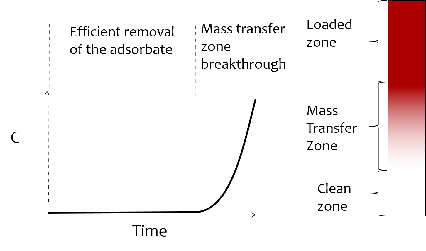
Fig. 18 Movie illustrating how the effluent concentration of the absorbate changes with time as the mass transfer zone moves through the fixed bed.

The velocity of the mass transfer zone (mtz or the adsorption front) can be obtained by a mass balance on the system. If we set our frame of reference (and our control volume) to be centered on the mass transfer zone, then the average velocity (over the pore fraction of the control surface) of fluid entering the mtz is equal to pore water velocity minus the velocity of the mtz. The fluid phase concentration of the adsorbate entering the control surface is \(C_0\) and the fraction of the control surface where fluid is passing through is the porosity, \(\phi\).

The average velocity of the solid phase exiting through the control surface is \(-v_{mtz}\). The bulk density of the adsorbate is \(\frac{q_0 M_{adsorbent}}{V_{column}}\). The mass rate of adsorbate passing through the control surface in liquid phase must precisely balance the mass rate of adsorbate passing through the control surface in the solid phase because the mtz is stationary.

(88)\[ [(v_{pore} - v_{mtz})C_0\phi] - \left[v_{mtz}\frac{q_0 M_{adsorbent}}{V_{column}}\right] = 0\]

We can apply continuity to find the relationship between the velocity in the pores and velocity above the porous fixed bed. The plan view area of the fixed bed cancels out.

(89)\[\phi v_{pore} = v_a\]

The effective bed porosity, \(\phi\) can be calculated from

(90)\[\phi =1 - \frac{\frac{M_{ac}}{\rho_{ac}} + \frac{M_{sand}}{\rho_{sand}}}{V_{column}}\]

where

\(\rho_{ac} = 2.1 g/cm^3\)

\(\rho_{sand} = 2.65 g/cm^3\)

Eliminate \(v_{pore}\) from the equation (88) we obtain:

(91)\[(v_a C_0 - v_{mtz}C_0\phi) - \left[v_{mtz}\frac{q_0 M_{adsorbent}}{V_{column}}\right] = 0\]

Now solve for \(v_{mtz}\).

(92)\[ v_{mtz}=\frac{v_a C_0}{C_0\phi + \frac{q_0 M_{adsorbent}}{V_{column}}}\]

In equation (92) the term \(C_0\phi\) represents the liquid phase mass of the adsorbate per unit volume of the fixed bed and the term \(\frac{q_0 M_{adsorbent}}{V_{column}}\) represents the solid phase mass of the adsorbate per unit volume of the fixed bed. The second term dominates for fixed bed adsorption reactors that are effective.

The time until breakthrough can be obtained by dividing the length of the adsorption column (\(L_{column}\)) by the velocity of the mtz (equation (92))

(93)\[\frac{L_{column}}{v_{mtz}} = \frac{L_{column}\phi}{v_a} + \frac{L_{column}q_0 M_{adsorbent}}{v_a C_0 V_{column}}\]

The equation above is equivalent to

(94)\[t_{mtz} = t_{water} + t_{ads}\]

Thus the time to breakthrough is the time required for water to flow through the reactor plus the additional time required due to the adsorption process. The retardation factor is defined as the ratio of the time for the mass transfer zone to travel through the bed divided by the time for water to travel through the bed.

(95)\[R_{adsorption} = \frac{t_{mtz}}{t_{water}} = \frac{v_{pore}}{v_{mtz}} = \frac{v_a}{\phi v_{mtz}}\]

Substituting equation (92) into equation (96) we obtain:

(96)\[ R_{adsorption} =1+ \frac{q_0 M_{adsorbent}}{C_0 \phi V_{column}}\]

Experimentally we can estimate \(R_{adsorption}\) based on the time required to reach 50% of the influent adsorbate for columns with and without adsorbent. Given the estimate of \(R_{adsorption}\) we can estimate the mass of adsorbate per mass of adsorbent, \(q_0\).

(97)\[ q_0 = \left(R_{adsorption} - 1\right) \frac{C_0 \phi V_{column}}{M_{adsorbent}}\]

From experiments conducted in the Cornell environmental laboratory around 2003 we have \(q_{50 mg/L}\) = 0.08. Our goal is to design a fixed bed reactor that has a \(t_{mtz}\) of about 30 minutes. With a 15 cm deep column at 1 mm/s and with a porosity of 0.4 the hydraulic residence time is 1 minute. Given a target retardation factor of 30 we can calculate the mass of carbon that we should have in the column. We can achieve this mass of carbon while holding the length of the column constant by diluting the activated carbon with sand.

The approach velocity for granular activated carbon contactors is generally between 1.4 and 4.2 mm/s. We will operate at 1 mm/s.

(98)\[ M_{adsorbent} = \left(R_{adsorption} - 1\right) \frac{C_0 \phi V_{column}}{q_0}\]

Different teams can try different masses of activated carbon or could experiment with filling the sand pores with coagulant as an alternative adsorbent.

""" importing """
from aguaclara.core.units import unit_registry as u
import aguaclara as ac
v_a = 1 * u.mm/u.s
porosity = 0.4
L_column = 15.2 * u.cm
D_column = 1*u.inch
A_column = ac.area_circle(D_column)
V_column = A_column * L_column
C_0 = 50 * u.mg/u.L
q_0 = 0.08
t_water = (L_column*porosity/v_a).to(u.s)
t_mtz_target = 1800*u.s
# set the breakthrough time to 30 minutes = 1800 s
R_adsorption = t_mtz_target/t_water
M_ac = ((R_adsorption-1)*C_0*porosity*V_column/q_0).to(u.g)
print('The mass of activated carbon given the dilution with sand should be',ac.round_sig_figs(M_ac,2))
Density_AC = 2100 *u.kg/(u.m**3)
#We measured the bulk density in the lab
Density_bulk_AC = 386 * u.kg/u.m**3
V_carbon = (M_ac/Density_bulk_AC).to(u.mL)
print('The volume of activated carbon is approximately',ac.round_sig_figs(V_carbon,2))
density_sand = 2650 * u.kg/u.m**3
M_sand = ((V_column-V_carbon)*density_sand*(1-porosity)).to(u.g)
print('The mass of sand is',ac.round_sig_figs(M_sand,2))

V_reddye = (v_a*A_column*t_mtz_target).to(u.L)
print('The volume of red dye required for one experiment is',ac.round_sig_figs(V_reddye,2))
Q_reddye = (v_a*A_column).to(u.mL/u.min)
print('The flow rate is',ac.round_sig_figs(Q_reddye,2))
mLperrev_Tubing_17 = 2.8 * u.mL/u.revolution
Pump_rpm = (Q_reddye/mLperrev_Tubing_17).to(u.revolution/u.min)
print('The pump rpm is',ac.round_sig_figs(Pump_rpm,3))

Contactor Procedures

The carbon contactor is set up to enable upflow or downflow and to select red dye or reverse osmosis water feeds. The flow directions are set using 3-way-valves. A 3-D model created by Ellie Beaudry, Harry Fuller, and Moriah Gilkey (2020) provides detail of the completed reactor assembly.

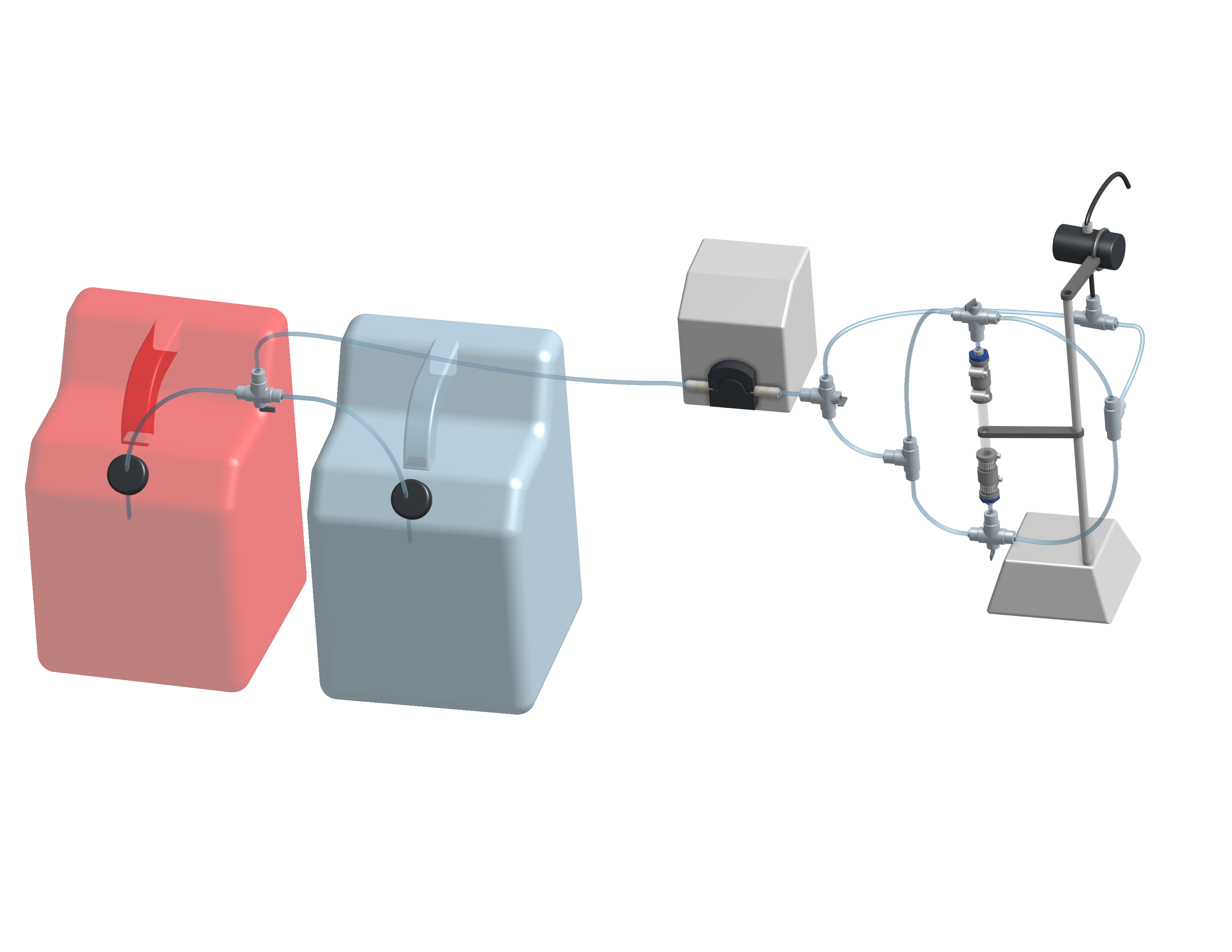
Fig. 19 Proposed design of the carbon column and feed system. The 3-D model is can be manipulated including setting the 3-way valves (Ellie Beaudry, Harry Fuller, and Moriah Gilkey 2020).

Carbon Contactor Setup

Assemble the system shown in Fig. 19. Use a peristaltic pump with #17 tubing at approximately 10 rpm. Prepare 20 L jerricans with 50 mg/L of Red dye #40. Use reverse osmosis water to dilute the dye. The carbon contactor will be operated in down flow mode. The specifications for the carbon contactors are given in Table Table 5.

Table 5 Carbon contactor settings.

Parameter	Value
Influent red dye Concentration	0.050 g/L
Mass of red dye/20 L	1.00 g
Depth of fixed bed	15 cm
Mass of sand	120 g (to fill column)
Approach velocity (1 mm/s)
Column diameter	2.54 cm
\(q_{(50 mg/L)}\)	0.080 g/g
Mass of carbon	5, 10, 15, 20 g

Set up the Contactor

Work through this procedure three times. For the first test skip the activated carbon and thus measure the F curve (see reactor modeling) for the sand column. Rinse the column with RO water, remove the sand, and repeat the procedure with a mixture of activated carbon and sand (see Table Table 5 for suggested masses of activated carbon).

1. Test column and pump and all tubing to ensure that it is leak tight using reverse osmosis water.
2. Verify that the photometer reads close to 0 mg/L while pumping reverse osmosis water.
3. Turn off pump.
4. Remove top from column
5. Mix sand and adsorbent (total volume of media adjusted to fill column)
6. Pour mixture of sand and adsorbent into a beaker containing reverse osmosis water (or tap water if using coagulant).
7. Swirl until most of the air is released.
8. Use a 50 mL syringe to remove about half of the water from the top of the column.
9. Use a funnel and a reverse osmosis water wash bottle to wash the mixture from the beaker into the column.
10. Use a 50 mL syringe to remove more water from the top of the column if necessary.
11. Use a long rod to gently stir activated carbon to help release air bubbles.
12. Assemble the column end fitting.
13. In up flow mode (at 0.5 mL/s), discharge the column effluent to waste until most of the fines are removed.
14. Next, run in down flow mode again and make sure to get all of the air out of the photometer.
15. Verify that the photometer is reading approximately 0 mg/L of red dye. This indicates that most of the activated carbon fines are removed from the column.
16. Configure ProCoDA to log the concentration of red dye at 5 second intervals
17. Switch the source valve from reverse osmosis to red dye solution and record a note that this is time zero.
18. Measure the flow rate using a balance to get mass of water in approximately 1 minute.
19. It is impractical to try and achieve \(C/C_0 = 1\), but run long enough to attain at least \(C/C_0 = 0.6\).

Troubleshooting and Reflections

We can anticipate several potential problems with this experimental design.

1. Air bubbles! Air in the sand column or in the photometer will result in failure. Surface tension makes it difficult to remove the air bubbles from the activated carbon. The methods may need to be modified if air causes problems.
2. Mass transport of the red dye into the activated carbon pores is slow because it is a diffusion process. It is possible that this will result in premature breakthrough of red dye long before the activated carbon reaches equilibrium with the influent concentration of red dye.
3. The relatively small amount of activated carbon in the sand column may result in inefficient transport of the red dye to the activated carbon granules. This would also result in inefficient removal of red dye.

An alternative to granular activated carbon is Poly aluminum chloride (PACl - not to be confused with Powdered Activated Carbon or PAC). PACl will remove red dye by adsorption and given that PACl forms nanoparticles (rather than millimeter sized granules for GAC) it is possible that the mass transport of red dye to PACl will be much faster than mass transport of red dye to GAC. This could be tested by substituting PACl for GAC in the column. We would need to develop a method to deliver the PACl flocs to the sand column.

Contactor Results and Analysis

1. Plot the breakthrough curves showing \(\frac{C}{C_0}\) versus time.
2. Find the time when the effluent concentration was 50% of the influent concentration and plot that as a function of the mass of activated carbon used.
3. Calculate the retardation coefficient (\(R_{adsorption}\)) based on the time to breakthrough for the columns with and without activated carbon.
4. Calculate the \(q_0\) for each of the columns based on equation (97). Plot this as a function of the mass of activated carbon used.

What did you learn from this analysis? How can you explain the results that you have obtained? What changes to the experimental method do you recommend for next year (or for a project)?

Prelab Questions

1. A carbon column is packed with 15 cm of activated carbon and then used to remove 50 mg/L of red dye #40. The approach velocity is 1 mm/s, the porosity is 0.8, and the bulk density of the activated carbon is 0.38 \(g/cm^3\). The mass of red dye per mass of carbon at equilibrium with 50 mg/L of red dye is 0.08. How long will it take for the mass transfer zone to travel to the bottom of the carbon column? This analysis shows why we use less activated carbon for our experiments in the lab!

Lab Prep Notes

Table 6 Reagent list.

Description	Supplier	Catalog number
activated carbon
red dye #40

Setup

1. Verify that all necessary supplies are in place for the pumps, tanks, column, valves, and tubing.
2. Prepare the Red Dye #40 stock solution.
3. Prepare a 5% bleach solution (5 mL bleach diluted to 100 mL with reverse osmosis water) for cleaning the photometer sample cell and sample lines.

Procedure to remove air from the top of the column

1. Close the Red Dye #40 influent valve.
2. Open the reverse osmosis water influent valve.
3. Wait for the influent line to clear of Red Dye #40.
4. Turn off the pump.
5. Reverse the column flow direction.
6. Turn on the pump until the air is removed.
7. Turn off the pump.
8. Reverse the column flow direction.
9. Turn on the pump and switch the influent to Red Dye #40.

References

Lawler, D. F., & Benjamin, M. M. (2013). Water quality engineering: physical / chemical treatment processes. Hoboken, N.J.: Wiley. Retrieved from http://search.ebscohost.com/login.aspx?direct=true&scope=site&db=nlebk&db=nlabk&AN=631668