Laboratory Measurements and Procedures
Introduction
Measurements of masses, volumes, and preparation of chemical solutions of known composition are essential laboratory skills. The goal of this exercise is to gain familiarity with these laboratory procedures. You will use these skills repeatedly throughout the semester.
Theory
Many laboratory procedures require preparation of chemical solutions. Most chemical solutions are prepared on the basis of mass of solute per volume of solution (grams per liter or moles per liter). Preparation of these chemical solutions requires the ability to accurately measure both mass and volume.
Preparation of dilutions is also frequently required. Many analytical techniques require the preparation of known standards. Standards are generally prepared with concentrations similar to that of the samples being analyzed. In environmental work many of the analyses are for hazardous substances at very low concentrations (mg/L or \(\mu g/L\) levels). It is difficult to accurately weigh a few milligrams of a chemical with an analytical balance. Often dry chemicals are in crystalline or granular form with each crystal weighing several milligrams making it difficult to get close to the desired weight. Thus it is often easier to prepare a low concentration standard by diluting a higher concentration stock solution. For example, 100 mL of a 10 mg/L solution of NaCl could be obtained by first preparing a 1 g/L NaCl solution (100 mg in 100 mL). One mL of the 1 g/L stock solution would then be diluted to 100 mL to obtain a 10 mg/L solution.
Absorption spectroscopy is one analytical technique that can be used to measure the concentration of a compound. Solutions that are colored absorb light in the visible range. The resulting color of the solution is from the light that is transmitted. According to Beer’s law the attenuation of light in a chemical solution is related to the concentration and the length of the path that the light passes through.
where c is the concentration of the chemical species, b is the distance the light travels through the solution, \(\varepsilon\) is a constant, \(P_o\) is the intensity of the incident light, and \(P\) is the intensity of the transmitted light. Absorption, A, is defined as:
In practice \(P_0\) is the intensity of light through a reference sample (such as deionized water) and thus accounts for any losses in the walls of the sample chamber. From equation (1) and (2) it may be seen that absorption is directly proportional to the concentration of the chemical species.
In this lab we will use a simple photometer with a 465 nm LED (blue light) and a detector that is used in smart phones to measure ambient light.
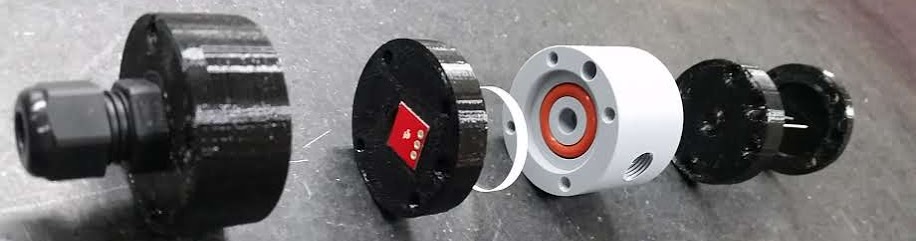
Fig. 2 Exploded view of the photometer. The LED is on the right and the sensor is on the red square printed circuit board. The flow path is through the gray PVC. Glass ports allow optical access to the sample.
Experimental Objectives
To gain proficiency in:
- Calibrating and using electronic balances
- Using signal conditioning boxes and data acquisition software
- Digital pipetting
- Preparing a solution of known concentration
- Preparing dilutions
- Measuring concentrations using a photometer
Experimental Methods
Mass Measurements
Mass can be accurately measured with an electronic analytical balance. Perhaps because balances are so easy to use it is easy to forget that they should be calibrated on a regular basis. It is recommended that balances be calibrated once a week, after the balance has been moved, or if excessive temperature variations have occurred. In order for balances to operate correctly they also need to be level. Most balances come with a bubble level and adjustable feet. Before calibrating a balance verify that the balance is level.
The environmental laboratory is equipped with 200 g balances. As part of this exercise, we will calibrate the 200 g as follows:
- Make sure the balance is stable and level using the bubble indicator
- Press and hold the cal button until the screen shows ‘cal’ briefly
- Wait until the screen flashes continually 100.000 g.
- Place the 100 g calibration mass on the pan (handle the calibration mass using a cotton glove or tissue paper)
- The scale is calibrated when it reads 100.000 g.
Dry chemicals can be weighed in disposable plastic “weighing boats” or other suitable containers. It is often desirable to subtract the weight of the container in which the chemical is being weighed. The weight of the chemical can be obtained either by weighing the container first and then subtracting, or by “zeroing” the balance with the container on the balance.
Temperature Measurement and ProCoDA
We will use a data acquisition system designed and fabricated in CEE at Cornell University. Each group has their own ProCoDA box and associated power supply and USB cable. The power supply and USB cable must be plugged into the ProCoDA box and then into the AC power on your lab bench and a USB port on your lab bench computer, respectively.
Use a thermistor to measure the temperature of reverse osmosis water. The thermistors are usually hanging on the rack to the right of the fume hoods (you should have one on your bench today). The thermistor has a 4-mm diameter metallic probe. Plug the thermistor into the red signal-conditioning box. The conditioned signal is connected to the ProCoDA box using a red cable. Connect the red cable to one of the sensor ports on the top row of the ProCoDA box.
- Open ProCoDA II and configure temperature monitoring
- Place the temperature probe in a 100-mL plastic beaker full of reverse osmosis water. Wait at least 15 seconds to allow the probe to equilibrate with the solution.
- Record this temperature in the attached spreadsheet.
Pipette Technique
- Use Fig. 3 or
density = pc.density_water(Temp)to estimate the mass of 990 \(\mu L\) of reverse osmosis water (at the measured temperature).- Use a 100-1000 \(\mu L\) digital pipette to transfer 990 \(\mu L\) of reverse osmosis water to a tared weighing boat on a balance with mg resolution. Record the mass of the water and compare with the expected value (see Fig. 3). Repeat this step if necessary until your pipetting error is less than 2%, then measure the mass of 5 replicate 990 \(\mu L\) pipette samples. Calculate the mean (\(\bar{x}\)), standard deviation (s), and coefficient of variation, \(\frac{s}{\bar{x}}\), for your measurements. The coefficient of variation (c.v.) is a good measure of the precision of your technique. For this test a c.v. \(\mathrm{<}\) 1% should be achievable.
Measure Density
- Weigh a 100 mL volumetric flask with its cap (use 200 g balance with resolution of 0.001 g}.
- Prepare 100 mL of a 1 M solution of sodium chloride in the weighed flask. You can also dissolve the NaCl in a clean beaker and transfer to the volumetric flask. Make sure to mix the solution and then verify that you have exactly 100 mL of solution. Note that the combined volume of NaCl and water decreases as the salt dissolves.
- Weigh the flask (with its cap) plus the sodium chloride solution and calculate the density of the 1 M NaCl solution.
""" importing """
from aguaclara.core.units import unit_registry as u
import aguaclara as ac
import matplotlib.pyplot as plt
import numpy as np

Temp = np.linspace(0,30)*u.degC
density = ac.density_water(Temp)
fig, ax = plt.subplots()
ax.plot(Temp,density)
ax.set(xlabel='Temperature (degrees Celsius)', ylabel=r'Density of water (kg/$m^3$)')
#fig.savefig('Laboratory_Measurements/Images/Density_vs_T')
plt.show()
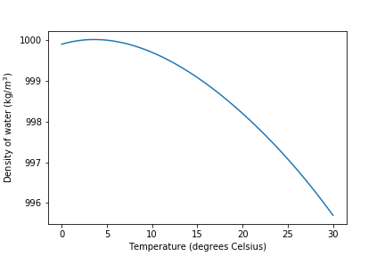
Fig. 3 Density of water vs. temperature.
Prepare red dye standards of several concentrations
A red dye stock solution of 10 g/L has been prepared.
- Use the red dye stock solution to prepare 100 mL of each of the following concentrations: 1 mg/L, 2 mg/L, 5 mg/L, 10 mg/L, 20 mg/L, 50 mg/L, and 100 mg/L. Record your calculations in the attached spreadsheet. Use pipettes and volumetric flasks to create accurate dilutions.
- Check all of the push to connect fittings in the photometer sample system. To obtain a water tight connection it is necessary to twist and push so that the o’ring slides over the outside of the tube to create a seal.
- Note any errors in transfer of mass as you prepare these dilutions (the color will make it easy to see). Make sure to transfer every drop!
Create a standard curve and measure an unknown
- Create a calibration curve using the standards created above and the photometer calibration method. Use the Sipper Cell Flow Calibration method. Tips: Use black opaque tubing on both ends of the photometer and remember to hold the photometer straight up. If you are getting odd readings on the photometer push the fluid back and forth the photometer using the syringe until the readings stablize. Tap the photometer lightly to remove any air bubbles.
- Make sure to both save AND export the calibration data from ProCoDA (
)
- Was the calibration linear? If not, which standards caused it to depart from linearity? #. The high concentration standards may be beyond the linear range for the sensor. This can occur if the amount of light reaching the sensor is too low to create an output voltage that is proportional to the light. Remember that an absorbance of 2 means that 99% of the light is adsorbed by the dye! If the absorbance for the highest standard isn’t in the line of the lower concentration samples, then delete the highest standards sequentially until you get a high correlation coefficient (R) as calculated by the ProCoDA photometer software. #. If the correlation coefficient is less than 0.99 then it suggests that your standards weren’t accurately prepared. See if you can identify what you did incorrectly with your pipette or dilution technique and consider (talk with a TA) preparing new standards.
- Save AND export the calibration data from ProCoDA (
- Measure the concentration of the unknown concentration of red dye. Note that you can do this directly in ProCoDA in the Graphs tab.
Clean Up
- Empty and rinse red dye bottles and place them on the drying racks
- Empty and rinse volumetric flasks and place them on the drying racks
- Place pipette tips in the pipette disposal mini cans
- Discard any used weighing boats
- Pull DI water through the photometer to rinse it and then place it in your drawer
- Rinse temperature probe and place it in your drawer
- Empty and rinse unknown red dye solutions
- Place concentrated red dye in your drawer
Prelab Questions
- You need 100 mL of a 1 \(\mu M\) solution of zinc that you will use as a standard to calibrate an atomic adsorption spectrophotometer. Find a source of zinc ions combined either with chloride or nitrate (you can use the internet or any other source of information). What is the molecular formula of the compound that you found? Zinc disposal down the sanitary sewer is restricted at Cornell and the solutions you prepare may need to be disposed of as hazardous waste. As an environmental engineering student you strive to minimize waste production. How would you prepare this standard using techniques readily available in the environmental laboratory so that you minimize the production of solutions that you don’t need? Note that we have pipettes that can dispense volumes between 10 \(\mu L\) and 1 mL and that we have 100 mL and 1 L volumetric flasks. Include enough information so that you could prepare the standard without doing any additional calculations. Consider your ability to accurately weigh small masses. Explain your procedure for any dilutions. Note that the stock solution concentration should be an easy multiple of your desired solution concentration so you don’t have to attempt to pipette a volume that the digital pipettes can’t be set for such as 13.6 \(\mu L\).
- The density of sodium chloride solutions as a function of concentration is approximately \(0.6985C + \rho_{water}\). What is the density of a 1 M solution of sodium chloride?
Data Analysis and Questions
Submit the spreadsheet containing the data sheet, and a markdown file containing graphs and answers to the questions.
- Fill out the attached spreadsheet. Make sure that all calculated values are entered in the spreadsheet as equations. All remaining analysis for the course will be done in Atom using Python!
- Create a graph of absorbance vs. concentration of red dye
\#40in Atom/Markdown using the exported data file. Does absorbance increase linearly with concentration of the red dye? Remove data points from the graph that are outside of the linear region (absorbance too high for the detector to measure accurately).- What is the value of the extinction coefficient, \(\varepsilon\)? Use the slope of the absorbance vs concentration to calculate the absorbance. The pathlength for the sample cell is given in the photometer section.
- Did you use interpolation or extrapolation to get the concentration of the unknown?
- What measurement controls the accuracy of the density measurement for the NaCl solution?
- What density did you expect (see prelab 2)?
- Approximately what should the accuracy be for the density measurement?
- Don’t forget to write a brief paragraph on conclusions and on suggestions using Markdown.
- Verify that your report and graphs meet the requirements as outlined on the course website.
Lab Prep Notes
Setup
- Prepare stock red dye #40 solution (10 g/L) and distribute to student workstations in 20 mL vials.
- Prepare 1 L of unknown in concentration range of standards. Divide into six 150 mL bottles (one for each student bench (teams/2)).
- Verify that balances calibrate easily.
- Disassemble, clean, and lubricate all pipettes.
- Distribute all supplies needed for the lab.